
Beneath the curve.
A CPU curve is the sum of thousands of optimizer decisions. PSG QX breaks it back down: which query, which plan, which place in the code, since when – and what every statement rests on.
- Layer 01 · SurfaceWhen did it change?The curve every monitoring tool shows.
- Layer 02 · PopulationWho carries the load?Many queries, but a few carry almost all of it.
- Layer 03 · MechanicsWhy did the optimizer decide this way?One plan, misestimated at one operator.
- Layer 04 · OriginWhere in the code?One line that makes the difference.
- Layer 05 · ImpactDid it help?Back at the surface: the curve is down again. Dashed: the trend before the change.
The question is simple: Did it get more expensive, or just more frequent? The answer isn't.
Monitoring reliably shows when a system gets slower. Why is not in the curve but in the executions beneath it: in plans, estimates, statistics, parameters and code. That is exactly where PSG QX comes in.
The same curve, read differently.
Drag the slider from the monitoring view to the QX view. The curve stays the same. It is only broken down into what it consists of.
Illustration with synthetic data, not a customer case.
Five layers beneath the curve.
Every investigation descends from the surface into the depth and returns with a verifiable statement.
-
Layer 01 · Surface
When did it change?
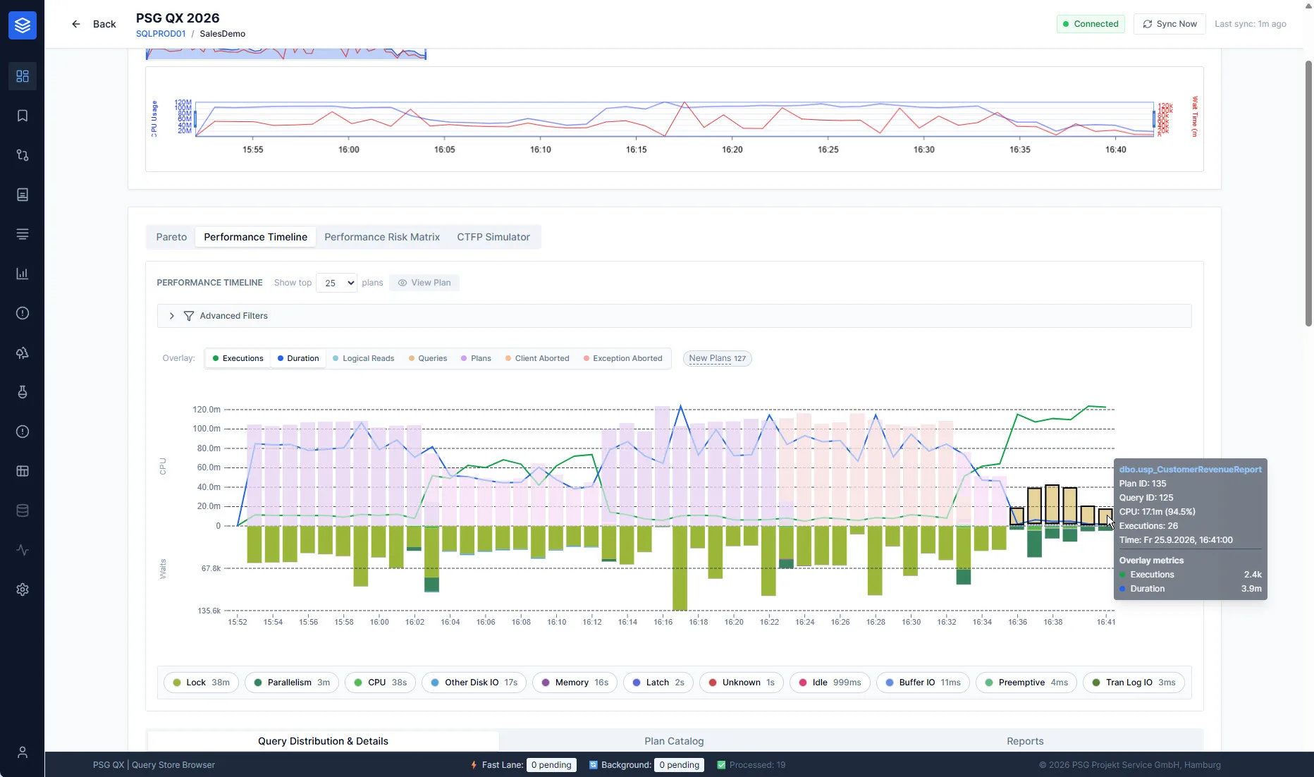
CPU, wait times and executions over time. Every monitoring tool offers this view. For us it is the starting point, not the result.
What the curve doesn't show: which query carries the load.
-
Layer 02 · Population
Who carries the load, and did it get more expensive or just more frequent?
Behind every interval are queries and their plans. QX shows which of them carry the load and whether a query ran more often or became more expensive per execution.
What the curve doesn't show: that two equally high spikes can have very different causes.
-
Layer 03 · Mechanics
Why did the optimizer decide this way?
Plans, estimates, statistics and parameters. This is where you see whether a known query has received a new plan, where estimate and reality diverge, or whether statistics were carried over from an earlier call.
What the curve doesn't show: that the optimizer worked with outdated assumptions.
What that looks like: One query, many plans →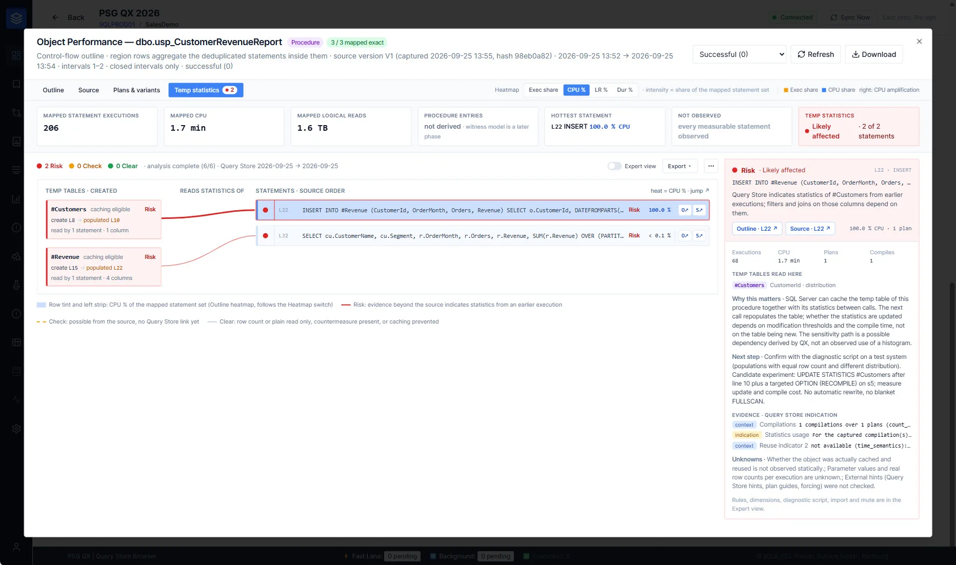
Finding from a demo workload: statistics of a temporary table from earlier calls. -
Layer 04 · Origin
Where in the code do we start?
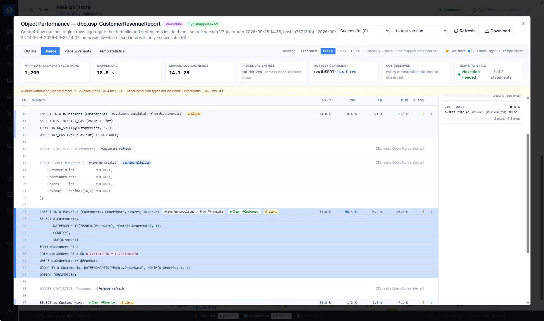
The load lands on the line in the procedure's source code, together with the plans that arose there. This turns a database finding into a task that development and operations can tackle together.
What the curve doesn't show: which line in the code causes the load.
-
Layer 05 · Impact
Did the change help?
Before and after under comparable conditions. Where conditions are not comparable, QX says so instead of claiming an improvement.
What the curve doesn't show: whether the lower load is due to the change or just to a quieter day.
Demo workload: After the change at 16:36, CPU per call drops while the number of calls rises.
The history as a data set, not a dashboard.
We read the execution history like data analysts: first check what the data supports, then draw conclusions. We have used data mining for this for years, long before generative AI and LLMs.
observation  CPU per call roughly tripled since Tuesday, calls unchanged.
in the plan  New plan for a known query; estimate far off at one join.
measured     More reads per call; the plan now runs in parallel but barely finishes sooner.
hypothesis   Statistics rebuilt after maintenance with a small sample.
open         Part of the load cannot be reliably assigned to a query and remains listed as such.
check        Update the statistics in a targeted way, compare the same metrics in the same time window.
Your own baseline instead of a rule of thumb
A phase is compared with earlier periods of the same pattern, not with a threshold from the manual.
Comparability first, then comparison
Every comparison is classified: comparable, limited or not possible, each with a reason.
Evidence levels
Confirmed in the plan, measured, or hypothesis. Observations are not presented as predictions.
Uncertainty stays visible
What cannot be assigned stays marked as such. Missing data does not count as zero.
Models have to prove themselves
Methods are tested against each other on the same history. A more elaborate model first has to show that it is better.
Local and repeatable
The analysis runs locally and without AI services. The same inputs and the same method version produce the same result.
The same question for over ten years.
PSG QX is the youngest generation of our own tools. The question behind it is older: What does a SQL Server workload actually do, and why?
- 2015Our own diagnostic toolsTalk at SQLBits about developing our own monitoring and diagnostic tools.
- 2017PSG MXMonitoring framework for continuous support, the first version in C#.
- 2020Machine learning for DBAsTalks on machine learning for DBA tasks and performance analysis; predictive monitoring from 2021.
- 2025PSG QXNew analysis core: the execution history, locally, from the timeline to the plan.
- 2026Down to the line of codeSource code, temporary tables and structured findings with evidence levels.
Tools can be built faster today than ever before. Which question to ask the data, and when a comparison doesn't hold, you only learn through real experience. Everything else is imitation.
Parallelism: rule of thumb or your own history?
“Cost threshold for parallelism at 50, MAXDOP at 8” – hardly any SQL Server setting has as many rules of thumb. Yet the right setting depends on what your workload actually does.
- Parallelism is a tool. In the right dose it makes large, critical queries finish much faster. In the wrong dose it burns CPU without anything finishing sooner.
- The goal is elapsed time, not wait time. A good setting spends the available CPU budget so that critical queries finish sooner in real elapsed (wall-clock) time.
- Waiting is part of it. Parallelism wait time occurs even when parallelism pays off. Tuning it down in isolation feels like action, but rarely makes anything faster.
What parallelism gains and costs
A parallel query distributes its rows across several threads and gathers them again at the end. This saves time for the query and costs the server additional CPU. Try out when it pays off.
Gate and width. Cost threshold for parallelism is the gate: it decides whether a query may get a parallel plan at all. MAXDOP is the width: how many cores it gets at most. Microsoft's recommendation by NUMA node derives that width from the hardware. For a generic server that is a reasonable starting value; for tuning it often falls short: MAXDOP then has to fit the workload, that is, how many queries compete for the same cores at the same time and which of them are critical. It's no coincidence that the width can also be set per database and with a query hint. The gate, by contrast, applies only to the whole instance.
Microsoft calls the default value of 5 for cost threshold for parallelism a starting point, not a recommendation
and advises changing it in small steps and observing a full business cycle each time. Microsoft Learn ↗
Simplified model for illustration, not a measurement.
What PSG QX makes of it
Instead of trying out every step for a full business cycle, QX re-evaluates the already recorded history under a different threshold. Explicitly as an observation, not a prediction.
- Vertical axis: the optimizer's cost estimate. The threshold decides on this alone.
- Horizontal axis: the CPU time actually measured.
- Red dashed line: the simulated threshold. Red points above it would be allowed to use a parallel plan.
- Hatched band: plans between the current and the simulated threshold. In the future they would be compiled serially.
- Filled or hollow: ran in parallel or serially. Point size represents the number of executions.
- Right: the effect in numbers, explicitly as an estimate based on the observed history.
Try it yourself
The same demo workload, simplified. Move the threshold and see which plans run in parallel today and would be compiled serially in the future.
Real metrics from a demo workload, shown in simplified form. Observed, not predicted: whether these plans would be faster or slower serially only becomes clear from a comparison after a change.
Cost versus reality
The threshold decides based on the optimizer's estimate, not on runtime. QX puts the two side by side.
What a change would cost
Which few queries benefit strongly from parallelism and would lose out under a blanket change?
Natural experiments
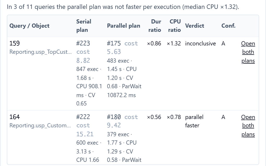
The same query ran once serially and once in parallel. What was actually faster?
When no setting helps
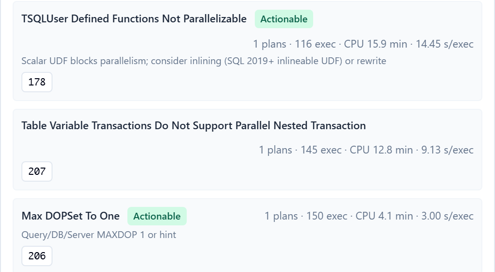
Expensive queries that run serially despite being suitable for parallelism, for example because of functions, hints or cursors. Here a change in the code helps, not a server setting.
Where QX fits into our work.
PSG QX is the tool our engineers use in troubleshooting, analysis and ongoing support. Typical occasions:
“It has been slower since the update.”
New queries, new and degraded plans, more frequent or more expensive: the comparison before and after the update.
To performance analysis → Urgent & PSG MX“It collapses at night, and in the morning everything is normal.”
The execution history shows the night after the fact. QX Recorder preserves evidence before it disappears.
More on performance → Development & vendors“The procedure is slow, but where?”
Statement and branch in the source code, temporary tables in the flow, the plans that go with them.
For software vendors → Infrastructure“More cores, but not faster.”
Which queries wait in parallel without getting faster, and what a different setting would have meant in your own history.
To infrastructure → Operations“The vendor says it's your database.”
A finding with plan and code location turns the question of blame into a factual conversation.
For MSPs & data center operators → Large environments“Many instances – where does the work pay off?”
How load and wait times are distributed across instances and databases.
For MSPs & data center operators →What PSG QX does not claim.
No automatic root cause
QX narrows things down and provides evidence. Whether a hypothesis is correct, we verify together with you.
No guaranteed speedup
A re-evaluation of the history shows what was observed, not what will happen in the future.
No substitute for experience
QX is our engineers' tool. People are accountable for the finding.
The analysis runs locally on the machine where QX runs, without cloud or AI services. Which data goes where, we define for each engagement. Already using PSG QX? Licenses and access →
Describe your case to us.
Which application, since when, how do you notice it? In the first conversation we clarify which data can answer your question. Please don't send any source code yet.